Introduction to Digital Images
Written November 25th, 2021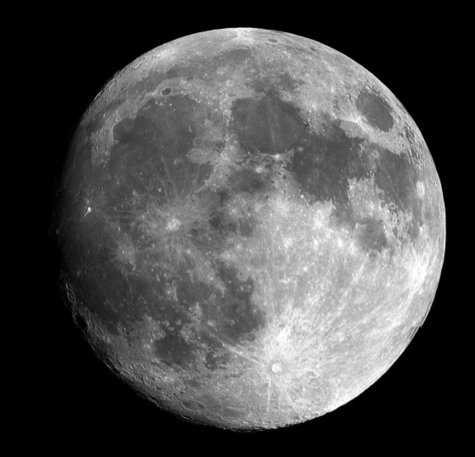 Above is the moon. It's a 8-bit grayscale image. To display the range of intensity values, I will use MATLAB to generate a histogram of the intensities.
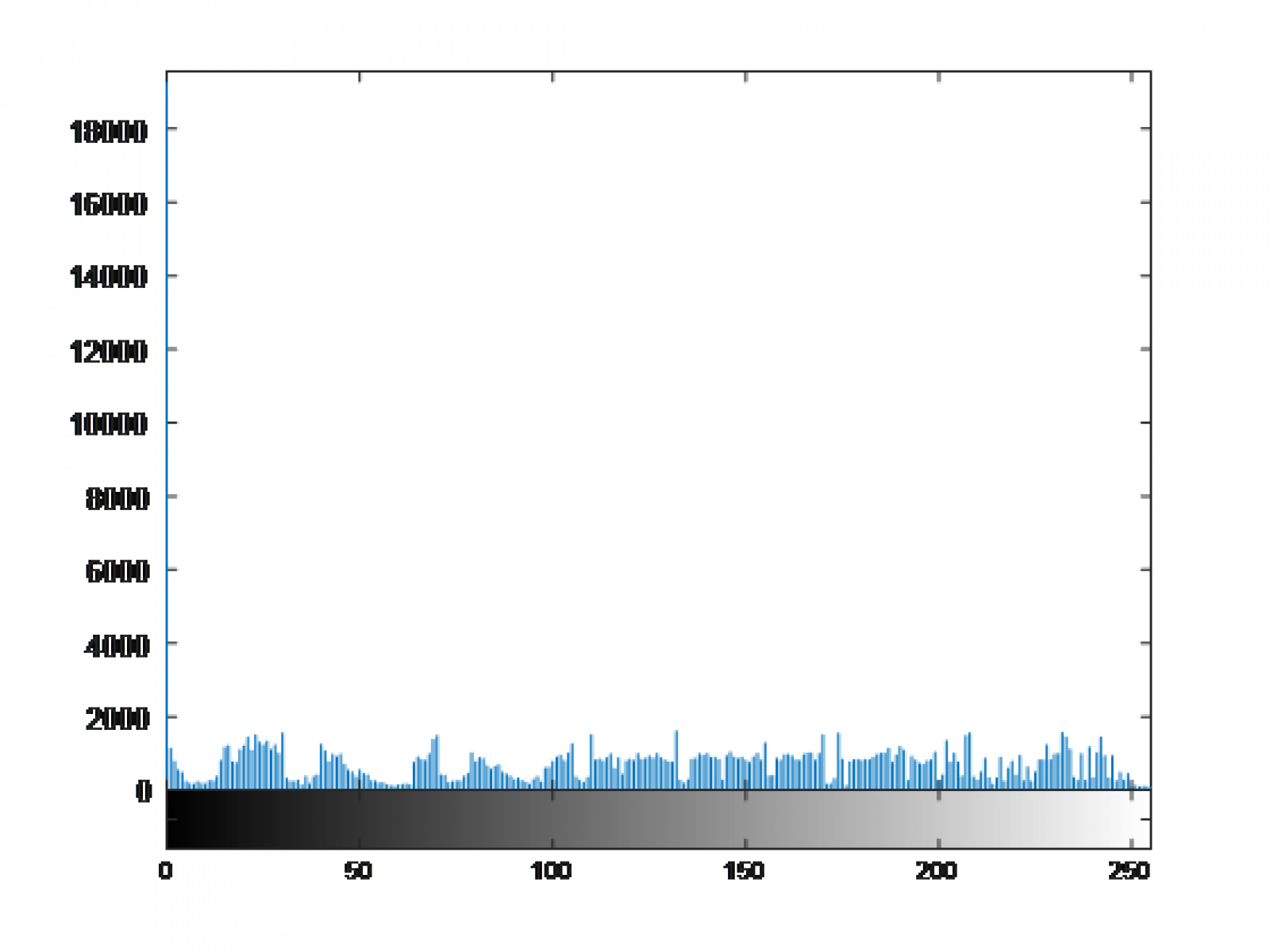 You can see the ranges in values from 0 to 255 but look at the distribution of values themselves - there is an enormous spike at an intensity of 0. For the sake of being thorough, it's the black background of the image. For some digital processing schemas, this might be an issue for detecting things.
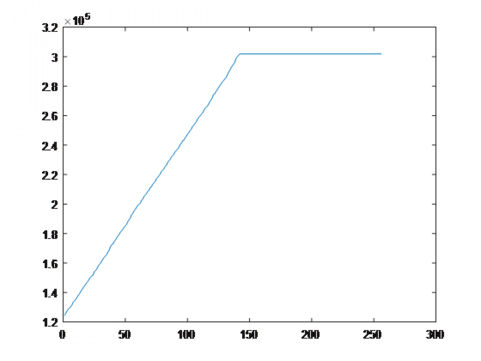
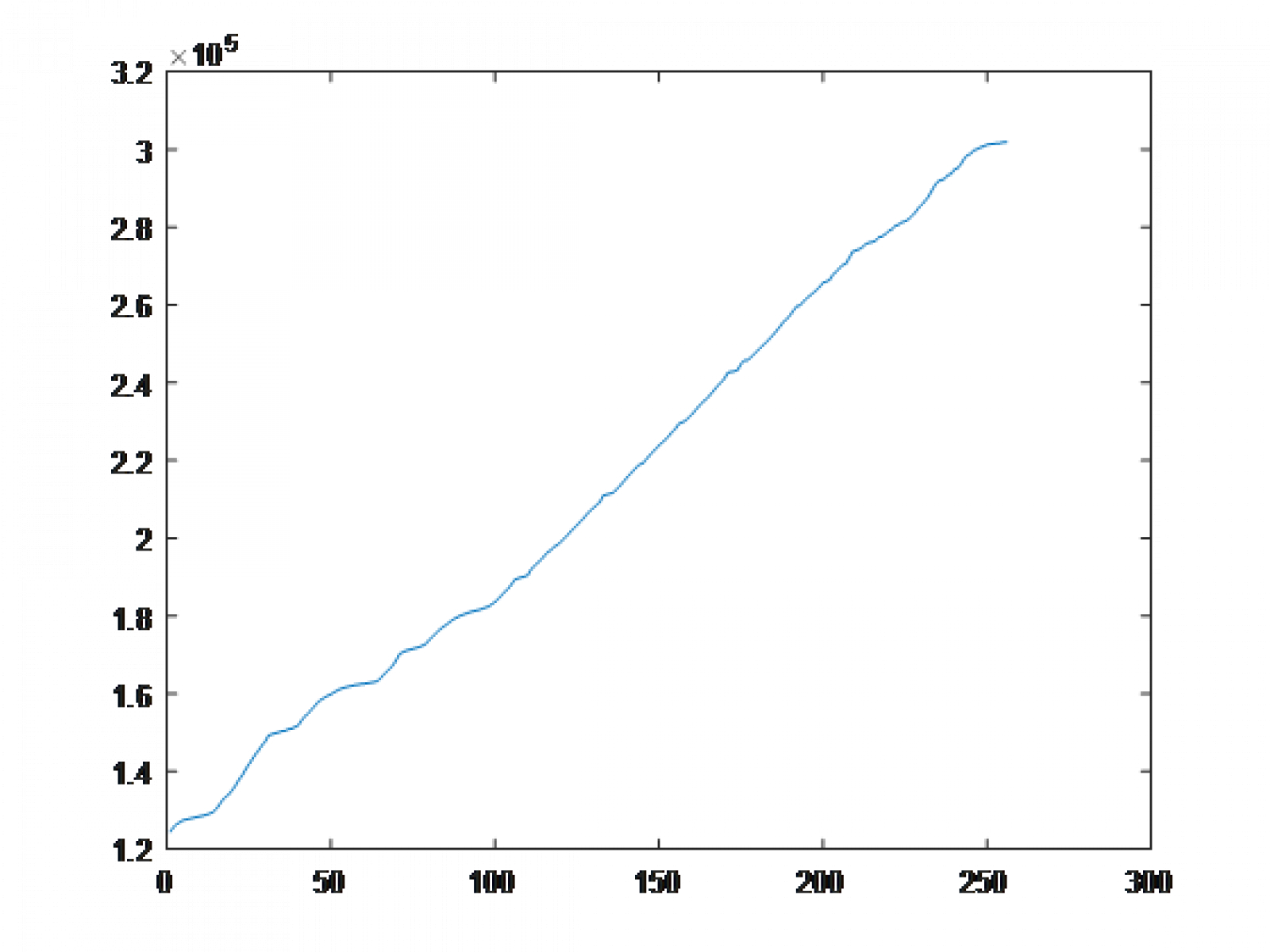 One thing that's important to notice is the vertical offset of the graph. This is another way that the analysis of image data indicates that the image has poor contrast. Thus, and ideally, an image of good contrast best approximates a line from an intensity of 0 to an intensity of 255 with a slope of the number of pixels over 255. This will become obvious as we work with the image more.Now, we start to introduce the transformation function T(r). Histogram equalization works by normalizing the CDF to the range of input/output values. This means that our transformation is the CDF above, but scaled in such a way that the input 0-255 maps to an output of 0-255.This is done because ideally, we want an equal weight on each intensity (turning the image histogram as close as possible into a uniform(a, b) random variable). So, if there is a spike in low intensities, the CDF favorites high intensities by selecting the higher range as the wider domain in <r>. Likewise, if an image favors high intensities, then the lower range of outputs has a greater domain in <r> and thus the CDF transformation favors mapping high intensities to low intensities. There are some examples on the wikipedia page for histogram equalization, near the bottom, if you are interested.After normalizing the CDF and inputting the moon image, this is the result. It is important to note that it doesn't look too good because the image already looked fine to the human eye.
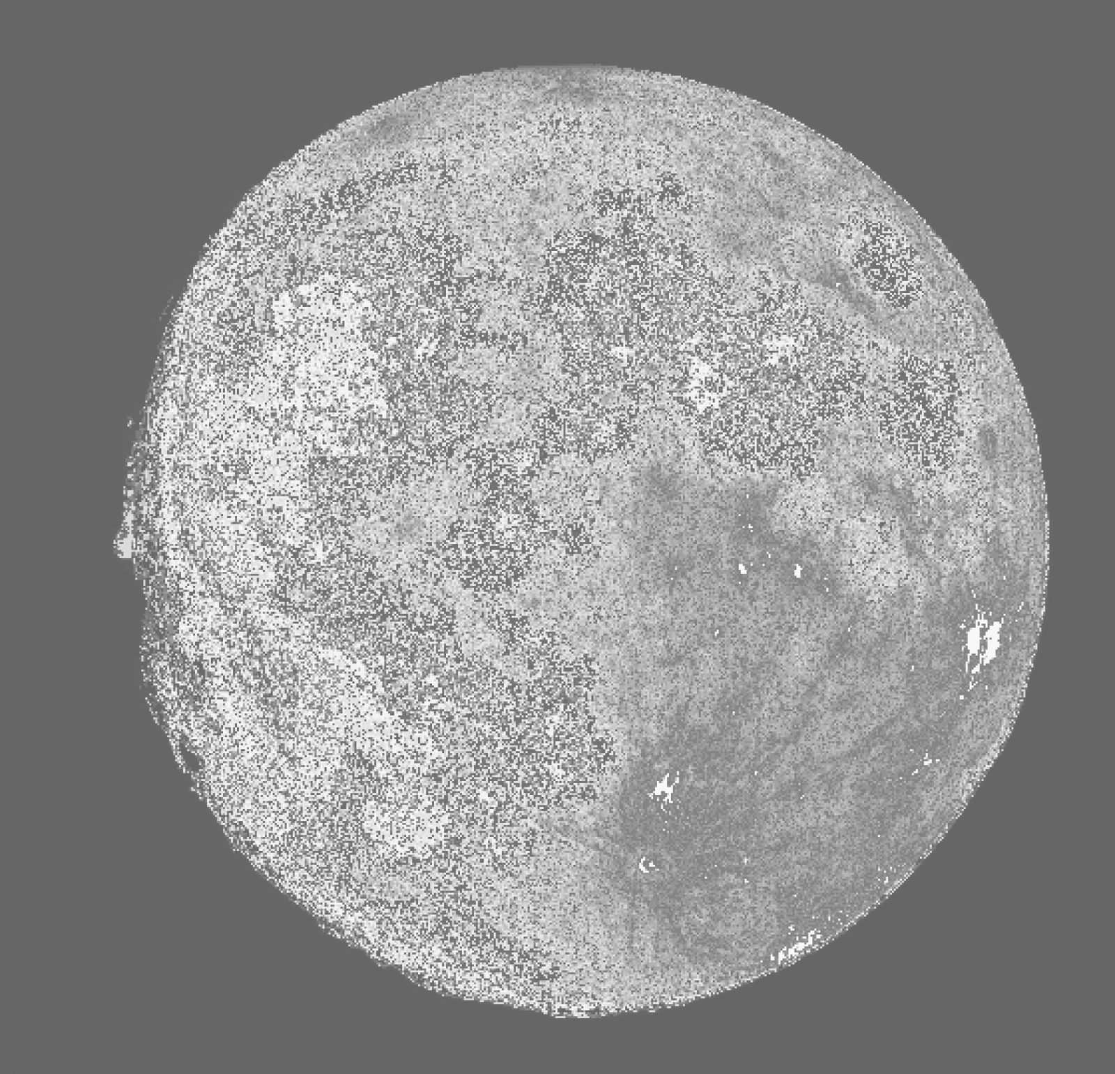 With the image, I also output the intensity histogram and the CDF of the output to show you how the transformations work.
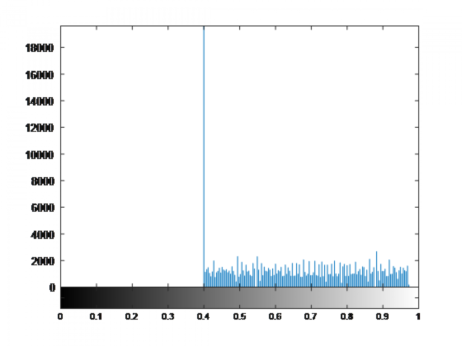
 You can see the attempt at creating a uniform random variable in the histogram, as well as the linearization in the CDF.With regards to the histogram, it is weighted rather evenly. If we consider the "space" taken up by the graph of each point, sort of like the expected value, then we should arrive at or close to the expected value of a uniform random variable. In this case, near 127.5. I didn't bother calculating this for time purposes - but it's another way to check your processor when undergoing histogram equalization.
Images, etc
Images are, of course, sets of visual data. Analog being photographs produced on film cameras, x-ray captures on various surfaces, and even paintings. Digital images are a much more different story in their makeup. Digital images are represented mathematically by an intensity function which takes in two spatial variables: [m]I(x, y).[/m][m]I(x, y)[/m] should be specified further to x being the horizontal spatial component and y being the vertical. However, digital images add a caveat in that they are discrete while [m]I(x, y)[/m] is a continuous function. Because of this, we need to introduce sampling. Most formats you'll find sampling in some form such as PPI, or pixels per inch. 1000 PPI means 1000 samples per inch, [m]1000^2[/m] per square inch. The following formula gives an explicit definition of a digital image including the sample distances [m]T_x[/m] and [m]T_y[/m] (inverse of the PPI, or sampling rate).[m]I[m, n] = I(xT_x, yT_y)[/m] where [m]0 \le m \le M-1[/m] and [m]0 \le n \le N-1[/m]This equation and conditions are the necessary conditions to work with and process digital images. There are M rows and N columns where any arbitrary discrete location (maybe a pixel, perhaps?) can be found at [m, n].The Basic Grayscale
The easiest type of image to work with is a grayscale image. You only have one value to work with at each pixel as opposed to RGB, which has three, and you can add one more if you include an alpha layer. With grayscales, you have a finite range of intensities that can be displayed to the user. Put formally, [m]0 \le I[m, n] \le I_{max} < \infin.[/m]First to note, the bounds of this function are from the physical nature of an image. Typically controlled by some property of the display you use: voltage or current signals cannot be infinite at a point. Second, the bounds are dependent on the range of intensities of the image itself. It has to be read somehow. One of the most common ranges of intensities is 8-bit, which means there are 256 discrete values [m]I[m, n][/m] could be at any given coordinate. However, the lowest value possible is an intensity of zero and thus the highest value possible is 255.Let's look at an example.Property: Contrast
Contrast, through the lens of this post, primarily deals with the distribution of intensities and how they are distributed. In the case of the image of the moon, it technically has rather poor contrast because of the spike at intensity equals zero (I say technically because the human eye can make out the features of the image rather well). For any digital image processor, contrast is one of the most important things to check for. So how do we change an image to fix its poor contrast while at the same time, keeping all the data of the image? The most straight-forward way to do this is a direct transformation given by the equation [m]s = T(r).[/m] <r> is a range of input intensities and <s> is the output intensity at any given pixelThis means that we are involving a basic form of convolution on the image with a kernel of dimensions (1, 1). I will make a post later covering convolution; if I don't, then please message me. However, assuming you are familiar with convolution, you will know that this means we iterate over every single pixel in the image. This convolution is aptly named "contrast equalization."The simplest transformation T(r) is a threshold function. If <r> exceeds some threshold, then the output is the maximum intensity, otherwise the output is the minimum intensity. Here is an interactive example on desmos. In this example, if <r> greater than or equal to 100, then the output <s> is 255 for the 8-bit interactive demo. Otherwise, <s> is 0. Fantastic.There are many other functions you can plot in the transformation space for our 1x1 kernel. It obviously gets more and more complex as you add inputs.Histogram Equalization
This is another basic - but powerful - method of equalizing contrast. So useful that MATLAB already has a function dedicated to it: histeq(img). For this method, we should take some time to learn what a Cumulative Distribution Function (CDF) is. It's a pretty horrifying topic in your average ECEN statistics class, but here it's not so bad. In short, the function is a summation of pixels up to each intensity value.[m]CDF F_I(i) = \sum_{j=0}^{i} r_j[/m] or, [m]F_I(i) = R[i \le r][/m].This function might be hard to think about, so let's look at the CDF of the moon image.So Why is it done?
I touched on this somewhere up above - but improving the relevant parts of your digital image processor never hurts. It can really only lead to good results in narrowing down the scope of what you're looking for in an image. One industry example of digital image processing is the work done on medical imagery before being analyzed. Another is microscopic imaging combined with computer vision. If there is an AI that can detect cancer, chances are you want it to see clearly.The scope of this post isn't very big. We only deal with simple kernels and change the contrast of an image. But with larger kernels, you can start to do things like a Gaussian blur, which is a weighted average of a square kernel. From that, you can also revert a Gaussian blur using kernels given you know the parameters. You can also deal with images that have multiple layers - RGB with or without alpha.However, at the bare minimum, it helps us see images better. I don't think that's a bad thing.Extra Resources
Here are some more resources to learn about histogram equalization and digital image processing:Dr. Timothy Schulz's youtube playlistDr. Jeff Jackson's lecture slides
New thread
Hello, my name is Yuval. I write a lot about food on here, but most of my actual work happens to involve imaging. I know a lot about Fourier Imaging Methods, Fourier Optics, and Deep Learning for Vision. Soon, I will be working on creating new LiDAR algorithms.Some of my work is available here: https://github.com/ylevental?tab=repositories